Solving a number game with a MIP solver
Table of Contents
1. The problem
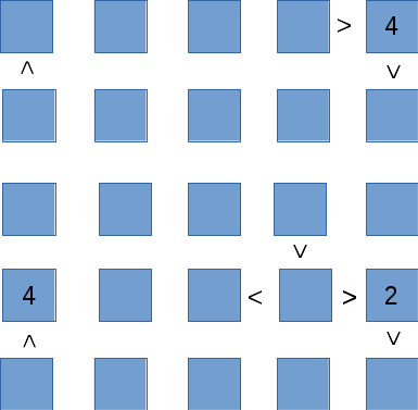
Consider the following puzzle: Chose numbers 1 to 5 such that in the diagram below each number is contained exactly once in each row and each column. The numbers in the fields should respect any inequality between two fields. We number the fields from the left top, e.g., field \((1,5)\) contains the number 4.
2. Finding a Solution
We will use pulp to solve this puzzle. The sudoku problem discussed in the pulp documentation provides some inspiration on how to tackle our problem.
from pulp import lpSum, LpVariable, LpMinimize
from pulp import LpProblem, LpStatus, value, LpInteger

prob = LpProblem("Number-Puzzle-Problem", LpMinimize)
3. The decision variables
As decision variables we use \(x_{kij}\) such that \(x_{kij} = 1\) if value \(k\) appears in the field with row \(i\) and column \(j\). The values, rows and columns are all elements of the set \(\{1, 2, 3, 4, 5\}\).
Vals = Rows = Cols =  range(1, 6)
x = LpVariable.dicts("x", (Vals, Rows, Cols), 0, 1, LpInteger)
4. Constraints with starting values
The simplest constraints deal with the numbers that are given in the diagram.
prob += x[4][1][5] == 1
prob += x[4][4][1] == 1
prob += x[2][4][5] == 1
5. Equality Constraints
There should be precisely one value in each field.
for r in Rows:
    for c in Cols:
        prob += lpSum([x[k][r][c] for k in Vals]) == 1
There can be only one value per row.
for k in Vals:
    for r in Rows:
        prob += lpSum([x[k][r][c] for c in Cols]) == 1
And also only one value per column.
for k in Vals:
    for c in Cols:
        prob += lpSum([x[k][r][c] for r in Rows]) == 1
6. Inequality Constraints
The inequality constraints of the board require more work.
Let's consider an example. In the problem diagram above we see that the value of field \((2,1)\) must be larger than the value in field \((1,1)\). Thus, if field \((2,1)\) has value 3, then field \((1,1)\) is not allowed to have a value of 3, 4, or 5. This means that, in terms of the decision variables, if \(x_{3,21}=1\) then \(\sum_{w=3}^5 x_{w,11} = 0\). More generally, we want that
\begin{equation} x_{k, 21} = 1 \Rightarrow \sum_{w=k}^5 x_{w, 11} = 0. \end{equation}We can implement this implication with the big \(M\) trick. Choose some big \(M\), then set
\begin{equation} \sum_{w=k}^5 x_{w, 11} \leq M(1-x_{k, 21}), \end{equation}so that if \(x_{k, 21} = 1\) then \(\sum_{w=k}^5 x_{w, 11}\) must be zero, while if \(x_{k, 21} = 0\), then \(\sum_{w=k}^5 x_{w, 11}\) is unconstrained. In code this becomes:
M = 100  # This is large enough

for k in Vals:
    prob += lpSum(x[w][1][1] for w in R[k:]) <= M * (1 - x[k][2][1])
In a similar way we implement the other inequalities.
for k in Vals:
    prob += lpSum(x[w][1][5] for w in R[k:]) <= M * (1 - x[k][1][4])
    prob += lpSum(x[w][2][5] for w in R[k:]) <= M * (1 - x[k][1][5])
    prob += lpSum(x[w][4][4] for w in R[k:]) <= M * (1 - x[k][3][4])
    prob += lpSum(x[w][4][1] for w in R[k:]) <= M * (1 - x[k][5][1])
    prob += lpSum(x[w][4][3] for w in R[k:]) <= M * (1 - x[k][4][4])
    prob += lpSum(x[w][4][5] for w in R[k:]) <= M * (1 - x[k][4][4])
    prob += lpSum(x[w][4][1] for w in R[k:]) <= M * (1 - x[k][5][1])
    prob += lpSum(x[w][5][5] for w in R[k:]) <= M * (1 - x[k][4][5])
A much simpler way (which occurred to me quite a bit later) is to define supplementary variables \(v\) that correspond to the value of the cell, i.e.,
\begin{equation} v_{ij} = \sum_{k=1}^5 k x_{kij}. \end{equation}Then we must have, for instance, for cells \((1,4)\) and \((1,5)\) that \(v_{14}>v_{15}\). In code this becomes
v = {}
for r in Rows:
    for c in Cols:
        v[(r, c)] = lpSum([k * x[k][r][c] for k in Vals])

prob += v[(1, 5)] <= v[(1, 4)]
prob += v[(1, 1)] <= v[(2, 1)]
prob += v[(2, 5)] <= v[(1, 5)]
prob += v[(4, 4)] <= v[(3, 4)]
prob += v[(4, 1)] <= v[(5, 1)]
prob += v[(4, 3)] <= v[(4, 4)]
prob += v[(4, 5)] <= v[(4, 4)]
prob += v[(4, 1)] <= v[(5, 1)]
prob += v[(5, 5)] <= v[(4, 5)]
Note that since all cells must have different values, all strict inequalities in the constraints can be implemented as a \(\leq\) constraints.
7. Objective
The objective is trivial, because there is nothing to optimize. We only use pulp to find a feasible solution.
prob += 0, "Arbitrary Objective Function"
8. Solving the problem
Solving the problem comes down to calling the solve() method of pulp.
prob.solve()
9. The solution
Have we found a solution?
print("Status: ", LpStatus[prob.status])
Status: Optimal
Yes! Let's print it.
for r in Rows:
    res = ""
    for c in Cols:
        for k in Vals:
            if value(x[k][r][c]) == 1:
                res += str(k) + " "
    print(res)
1 2 3 5 4
2 4 5 1 3
3 1 2 4 5
4 5 1 3 2
5 3 4 2 1