Metropolis-Hastings Algorithm

The first time I read about the Metropolis-Hastings (MH) algorithm I found it all very confusing. The reason is that I was (am?) used to think in terms of Markov chains and transition matrices, and then the goal is to find the stationary distribution \(\pi\). In the Metropolis-Hastings algorithm, the situation is precisely reversed: for a given distribution \(\eta\), say, construct a Markov chain whose stationary distribution is \(\eta\). My first point of confusion with this was: why do this, if we already have \(\eta\)? Then I read on, to discover that the MH algorithm is used to compute the normalizing constant for some distribution \(\eta\). Ok, but why? If I start with a Markov chain, then I have no clue about the functional form of \(\pi\). What then does it help to try to find its normalizing constant when the only thing that I have available is the transtion matrix?

So far my misconceptions. After reading yet more, I finally discovered that the MH algorithm is used for distributions whose functional form is completely known, but only the normalizing constant is too hard to compute. In other words, we just use the MH algorithm to estimate the normalizing constant by means of simulation.

An example for which the functional form of the stationary distribution is known is the distribution of jobs in a closed queueing network consisting of \(N\) \(M/M/1\) stations.

Here is an example in python code to demonstrate how all this works. I learned it here.

We start with the regular

import matplotlib.pyplot as plt
import numpy as np
import scipy.integrate as integrate

# from latex_figures import *

gen = np.random.default_rng(3)

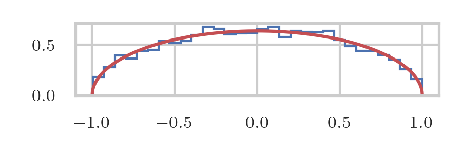
Suppose we are given as unnormalized density the function \(p(x) = \sqrt{1-x^{2}}\) with a support on \([-1,1]\). Clearly, this is the half circle, and its normalization factor is \(Z=\pi/2\). We define \(Z\) here, but don't use it in the simulation because there we are supposed not to know this normalization factor.

def p(x):
    return np.sqrt(1 - x**2)


Z = np.pi / 2

We next run the MH algorithm. I implicitly assume that the Markov chain that is used is symmetric, so that it falls out of the equations. Observe, it is not my aim to explain the details of the MH algorithm, but just how it works. Once you understand that the MH algorithm is meant to be used to sample from a given unnormalized density function, the rest is quite easy to understand.

Since the support of \(p\) is \([-1,1]\), I use a uniform rv on \([-1,1]\) to provide a candidate solution \(x'\). When the system is in state \(x\), the acceptance probability becomes \(p(x')/p(x)\). As explained in the literature, it is best to drop the first samples, i.e., to wait for a certain burn-in time.

N = 10000
samples = np.zeros(N)
xt = 0.0
for i in range(len(samples)):
    xt_candidate = gen.uniform(-1, 1)
    if gen.uniform() < p(xt_candidate) / p(xt):
        xt = xt_candidate
    samples[i] = xt
burn_in = len(samples) // 10
samples = samples[burn_in:]

So, now we have a set of samples that we can use for estimation purposes. Let us first compare the probabilities we obtained with the theoretical values by making a histogram. The conversion of a bin heights in a histogram to estimates of the pmf is a bit tricky; at least, I did not directly see how to do it, so here is the reasoning in full. Suppose we have samples \(\{X_{i}\}_{i=1}^{N}\), then the height of a bin, with the interval \(A\) as support, is just the number of samples that hit \(A\), i.e.,

If the length of \(A\) is small, then, \(c(A) \approx N p(x) |A|\) where \(p(x)\) is the density \(p\) computed at the midpoint \(x\) of \(A\). Thus, if we want to estimate \(p(x)\) based on the histogram, then

where \(|A| = 2/n\) when the interval \([-1,1]\) is chopped up into \(n\) bins.

n_bins = 30
counts, bins = np.histogram(samples, bins=n_bins)
dx = 2 / n_bins
pmf = counts / sum(counts) / dx
midpoints = (bins[:-1] + bins[1:]) / 2

Let's compare our estimates to the theoretical values. Here we use \(Z\) to scale \(p\) to the proper values; once again, note that we did not use \(Z\) in the simulations.

x_vals = np.linspace(-1, 1, 1000)
y_vals = p(x_vals)

plt.figure(figsize=(3, 1))
plt.plot(x_vals, y_vals / Z, 'r', label='P(x)')
plt.stairs(pmf, bins)
plt.tight_layout()
plt.savefig("../images/MH-half-circle.png", dpi=300)

We can use the midpoints and the histogram to estimate the normalization factor \(Z\) by comparing the counts to the probabilities at the midpoints.

true_probs = np.array([p(k) for k in midpoints])
Z_estimates = true_probs / pmf
print(f"{Z_estimates.mean()=:2.3f}, {Z=:2.3f}")

Z_estimates.mean()=1.589, Z=1.571

This is not bad at all.

Finally, we actually don't need \(Z\) at all to estimate the expected values of functions.

f = lambda x: x**2
E_f = integrate.quad(lambda x: f(x) * p(x) / Z, -1, 1)[0]
E_f_estimated = np.mean(f(samples))
print(f"{E_f_estimated=:2.3f}, {E_f=:2.3f}")

E_f_estimated=0.247, E_f=0.250

And this is also a nice result.

Perhaps I add at a later stage how to estimate the distribution of jobs in a closed queueing network.