We implement in Sagemath manifolds the computations for the twin problem¹¹ When a twin can undergo instantaneous changes in speed, Bondi’s \(k\)-calculus provides a simpler framework. as discussed in Chapter 2 of Gourgoulhon, Relativité restreinte.²² Or the English version: Gourgoulhon, Special Relativity in General Frames. We expect that the reader of the code ³³ This link offers further examples for Sagemath and differential geometry. below has a copy of this book at hand. When referring to, for instance, equation (2.1) of this book, we write (G.2.1).

We first need a 2D Minkowski space with coordinates \(t\) and \(x\).⁴⁴ The Black python code formatter hangs on X.<c,t>. I therefore instantiate the chart slightly differently.

M = Manifold(2, 'M', structure='Lorentzian')
X = M.chart(names=("t", "x"))
t, x = X[:]
# X.<t,x> = M.chart() # the black formatter does not like this syntax

Next is the metric.

g = M.lorentzian_metric('g', signature='positive')
g[0, 0], g[1, 1] = -1, 1
show(g.disp())
show(g.signature())

\[ g = -\mathrm{d} t\otimes \mathrm{d} t+\mathrm{d} x\otimes \mathrm{d} x \] \[ 0 \]

Here is the \(x\) coordinate of the path \(\mathscr{L}'\).

c, alpha, T = var('c alpha T', domain='positive')
x = c * T / alpha * (sqrt(1 + (alpha * t / T) ^ 2) - 1)
show(x)

\[ \frac{T c {\left(\sqrt{\frac{\alpha^{2} t^{2}}{T^{2}} + 1} - 1\right)}}{\alpha} \]

With this, we build the part of the path \(\mathscr{L}'\) from the point \(A\) at which the twins separate to the point \(C\) at which the twin that is flying hits the brakes to slow down; we skip the other three parts of \(\mathscr{L}'\).⁵⁵ They follow from symmetry.

Lp = M.curve(
    [c * t, x],
    (t, 0, T / 4),
    chart=X,
    name='Lp',
)
show(Lp.display())

To plot \(\mathscr{L}'\) we need to choose numerical values for \(T\), \(\alpha\), and the speed of light \(c\). We achieve this by substituting the numerical values in \(x\), and then defining a new curve with these values.

x_of_t = x.subs({alpha: 8, T: 5, c: 1})
Lp_plot = M.curve(
    (x_of_t, t),
    (t, 0, 5 / 4),
)
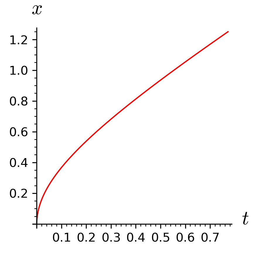
p = Lp_plot.plot()
p.save("twins_curve.png", figsize=(3, 3), dpi=300)

The figure below shows the worldline of the twin that is undergoing the accelerations.⁶⁶ The axis labels do not follow the convention of special relativity to have \(t\) pointing upward and \(x\) sideways. For the moment, I don’t know how to repair this.

For the infinitesimal proper time \(\d \tau\) we have from (G.2.9)

where \(\mathbf{v}\) is a tangent vector of the path parametrized by \(t\). Thus, we need to compute the tangent vector \(\mathbf{v}\) first.

v = Lp.tangent_vector_field(name='v', latex_name='\\mathbf{v}')
show(v.display())

\[ \mathbf{v} = c \frac{\partial}{\partial t } + \left( \frac{\alpha c t}{\sqrt{\alpha^{2} t^{2} + T^{2}}} \right) \frac{\partial}{\partial x } \]

For the dot product \(\mathbf{v} \cdot \mathbf{v}\) we have to pullback the metric from \(M\) to \(\mathscr{L}'\).

d_tau = sqrt(-g.along(Lp)(v, v)) / c
show(d_tau.disp())

The proper time of the first quarter of the total curve from leaving to returning is \(\tau = \int_0^{T/4} \d \tau\):

Tp = integral(d_tau.expr(), t, 0, T / 4)
show(Tp/T)

\[ \frac{\operatorname{arsinh}\left(\frac{1}{4} \, \alpha\right)}{\alpha} \]

From \(\mathbf{v}\) we compute the \(4\)-velocity \(\mathbf{u} = \mathbf{v} /|| \mathbf{v} ||\).

u = v / v.norm(g.along(Lp))
show(u.disp())

\[ \left( \frac{\sqrt{\alpha^{2} t^{2} + T^{2}}}{T} \right) \frac{\partial}{\partial t } + \frac{\alpha t}{T} \frac{\partial}{\partial x } \]

Note that the next two ways of computing the norm are the same.

show(v.norm(g.along(Lp)) == sqrt(-g.along(Lp)(v, v)))

\[ \mathrm{True} \]

The \(4\)-acceleration is defined as

We first compute \(\d \mathbf{u}/\d t\).

du_dt = Lp.tangent_vector_field(latex_name='\\d u/\\d t')
for i in M.irange():
    du_dt[i] = diff(u[i].expr(), t)

show(du_dt.disp())

\[ \d u/\d t = \left( \frac{\alpha^{2} t}{\sqrt{\alpha^{2} t^{2} + T^{2}} T} \right) \frac{\partial}{\partial t } + \frac{\alpha}{T} \frac{\partial}{\partial x } \] The \(4\) acceleration now follows simply.

a = du_dt / (c * d_tau)
show(a.disp())

\[ \frac{\alpha^{2} t}{T^{2} c} \frac{\partial}{\partial t } + \left( \frac{\sqrt{\alpha^{2} t^{2} + T^{2}} \alpha}{T^{2} c} \right) \frac{\partial}{\partial x } \]

Here are some further checks: \(\mathbf{u}\cdot \mathbf{u}\) should equal \(-1\), and \(\mathbf{u}\cdot \mathbf{a} = 0\).

show(g.along(Lp)(u, u).disp())
show(g.along(Lp)(u, a).disp())

Finally, let’s check that \(\mathbf{a}\cdot \mathbf{a}\) corresponds to \(\alpha^2/c^{2} T^{2}\).

show(g.along(Lp)(a, a).disp())

This code facilitates the export to \(\LaTeX\).

def show(s):
    s = latex(s).rstrip()
    res = r"\["  # \begin{dmath*}"
    res += "\n" + s + "\n"
    res += r"\]"  # end{dmath*}"
    print(res)