The FFT is actually a super fast algorithm to find the probability mass function (pmf) of the sum of two independent discrete rvs. To see it’s value, we start with a simple example.

Consider two rvs \(X, Y\) both with outcomes in \(\{0, \ldots, N-1\}\) and pmfs \(p_{X}\) and \(p_{Y}\). A simple procedure to compute the distribution of the sum \(Z=X+Y\) is by means of conditioning:

Such a sum over terms \(a_{n-k}b_{k}\) where \(a_{n-k} = p_Y(n-k)\) and \(b_k = p_X(k)\) is called a convolution of the series \(\{a_k\}_{k=0}^n\) and \(\{b_k\}_{k=0}^{n}\). Here is the code to compute \(p_{Z}\).

from collections import defaultdict

px = py = [1, 1, 1]  # unnormalized
pz = defaultdict(float)

for i in range(len(px)):
    for j in range(len(py)):
        pz[i + j] += px[i] * py[j]

Observe that we need two nested for loops. This becomes very slow when \(N > 10^{3}\) or so.

A fast way can be found by using moment-generation functions (mgfs). To see how this might help, we use the following idea. To uniquely fix a constant, i.e., a 0-degree polynomial, we just need the value of this polynomial at one point. For a line, i.e., a 1-degree polynomial, we need the value at two points. For a parabola, i.e., a 2-degree polynomial, we need three points. In general, there is a theorem that states that by specifying \(N\) points we can fix a polynomial with degree \(N-1\).

If we expand the mgf of the rv \(X\), we obtain

because the pmf of \(X\) is concentrated on \(N\) points. Clearly, \(M_X\) is a \(N-1\)-degree polynomial in \(x=e^{s}\). By the same argument, \(M_Y\) is also a polynomial of degree \(N-1\). Therefore

is the product of two \(N-1\) degree polynomials. Consequently, \(M_{Z}\) must be a polynomial of degree \(2(N-1)\). Thus, to characterize \(M_{Z}\) we need \(2 (N-1) + 1 = 2N - 1\) points. In other words, if we know the values \(M_X(z_k)\) and \(M_Y(z_k)\) at points \(z_{k}, k=0, \ldots 2N-1\), then the \(2N-1\) values \(M_Z(z_k) = M_X(z_k) M_Y(z_k)\) should fix the coefficients of \(M_{Z}\) uniquely. And since computing \(M_{Z}\) at the \(2N-1\) points \(z_0, z_{1}, \ldots, z_{2N-1}\) involves \(2N-1\) multiplications, this is an \(O(N)\) procedure.

So, to benefit from an \(O(N)\) procedure, we need to know the complexity to compute \(M_{X}\) and \(M_Y\) at \(2N -1\) points \(\{z_{k}\}\). A naive method to compute the mgf of the rv \(X \sim\Unif{\{1, 2, 3\}}\) on the points \(z=1, 2, 3, 4, 5\) is like this.

import numpy as np

px = [1 / 3, 1 / 3, 1 / 3]
z = [1, 2, 3, 4, 5]
mx = [0] * len(z)
for n in range(len(z)):
    for k in range(len(px)):
        mx[n] += np.exp(z[n] * k) * px[k]

But observe that this method has \(O(N^2)\) complexity, so it appears that we have gained nothing.

However, with a very clever choice of points \(z_k\) there exists an \(O(N\log N)\) algorithm to compute \(M_X\) at \(N\) points. Moreover, the same algorithm can be used to invert \(M_{Z}\), that is, we can retrieve the probabilities \(p_{Z}(k), k=0, \ldots, 2N-1\) from the values \(M_Z(z_k), k=0, \ldots 2N-1\) also in \(O(N\log N)\) time. This algorithm is the fast Fourier transform which we discuss now. ¹¹Part of the material here is based on my favorite book on algorithms: Introduction to Algorithms, by T.H. Cormen, C.E. Leiserson, R.L. Rivest.

To understand the basic workings of the FFT we just need Euler’s formula \(e^{i \pi} = -1\) where \(i=\sqrt{-1}\).

The FFT consists of three steps. The first important idea is to focus on the set of points \(s_k=2\pi i k/N\), rather than a general set of points, and take \(N\) a power of \(2\). With this,

The second step is very simple. Split the polynomial \(M_{X}\) into two polynomials, one with the even terms, the other with odd terms:

Thus, \(E\) and \(O\) represent the even and odd terms of \(M_{X}\) and both are polynomials of degree \(N/2\) rather than \(N\).

The third trick is also simple, but its importance is somewhat hard to realize. Write \(k' = k + N/2\), then

where we use Exercise 1. This implies that \(E(s_{k+N/2}) = E(s_k)\) and \(O(s_{k+N/2}) = O(s_k)\). With this we can see that for \(k=0, \ldots, N/2-1\),

and on \(k'=N/2, \ldots, N-1\),

Hence, we only have to compute \(E\) and \(O\) on \(N/2\) points \(s_k\) to retrieve \(M_X\) at \(N\) points! The last step is to realize that we can apply this procedure recursively to \(E\) and \(O\), until the recursions reach 0-degree polynomials, which are just constants.²²For some further interesting discussion: https://jakevdp.github.io/blog/2013/08/28/understanding-the-fft/.

If you recall how quicksort works, then you’ll realize immediately that the FFT has complexity \(O(N\log N)\) rather than \(O(N^2)\).

With the work above, the code for the FFT is now simple. There is one detail: the FFT is defined in terms of \(M_X(-s)\) instead of \(M_X(s)\). For that reason we need to include a minus sign in the factor f in the code. Next, in python 2j represents the imaginary number \(2i\). The last line is just a check on the correctness.

import numpy as np


def FFT(x):
    """A recursive implementation of the 1D Cooley-Tukey FFT"""
    x = np.asarray(x, dtype=float)
    N = len(x)

    if N == 1:
        return x
    elif N % 2 > 0:
        raise ValueError("size of x must be a power of 2")
    else:
        E = FFT(x[::2])  # even
        O = FFT(x[1::2]) # odd
        f = np.exp(-2j * np.pi * np.arange(N / 2) / N) # factor
        return np.concatenate([E + f * O, E - f * O])


gen = np.random.default_rng(3)
x = gen.uniform(0, 1, 1024)
print(np.allclose(FFT(x), np.fft.fft(x)))

The inverse FFT works equivalently. Given a set of numbers \(\{z_{k}\}_{k=0}^{2N-1}\), the inverse is defined as

We leave the rest to the reader.

While the above illustrates the basic principles of FFT, it is better not to use it for real problems. Industry strength implementations, such as the one in numpy, use decennia of smart ideas to improve the speed and robustness of the algorithm. For this reason we use np.fft.fft henceforth.

Let us demonstrate how to use the FFT to find the distribution of the sum \(Z\) of two uniform dice each with sides \(\{0, 1,\ldots, 5\}\). Note that \(\min Z= 0\) and \(\max Z = 10\); we should compute \(M_{X}\) and \(M_{Y}\) on at least \(6+6-1\) points, and don’t take the real part of the FFT.³³I made both errors initially.

px = np.ones(6, dtype=float)
px_hat = np.fft.fft(px, n=2 * len(px) - 1)
pz_hat = px_hat * px_hat  # multiply pointwise
pz = np.fft.ifft(pz_hat).real

With the FFT we can now develop code to smoothen a histogram by means of KDE.⁴⁴I am not particularly fond of using KDEs, see here. However, FFT is a nice tool, so let’s just demonstrate its use. Suppose we have observed outcomes \(x_1, x_2, \ldots, x_n\) of some rv \(X\) and we want to use a kernel \(K_h\) to estimate the density at a some point \(x\):

If we concentrate on a grid \(u_{k} = u_0 + h k\), for \(h\) small and \(u_0\) some reference point, then,

where \(n_j\) is the number of outcomes in the interval \([u_j, u_j + h)\). Clearly, \(u_{k}-u_j = (k-j)h\), hence, \(K_h(u_k-u_j) = K_h((k-j)h)\). If we write \(a_{k-j} = K_{s}((k-j)h)\), then,

But now observe that this \(f\) is a convolution! And this opens the door to using FFT as a fast method for smoothing.

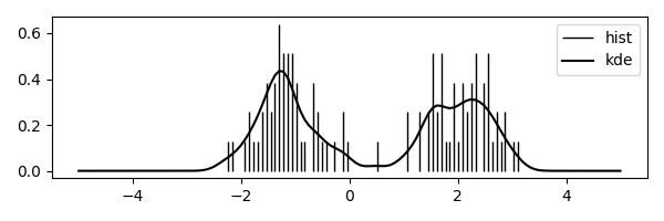
Here is the code; Fig. 1 shows the result.

import numpy as np
import matplotlib.pyplot as plt
from scipy.stats import norm

np.random.seed(3)

N = 50
# Make a camel shaped density
X = np.r_[norm.rvs(size=N, loc=-1, scale=0.5), norm.rvs(size=N, loc=2, scale=0.5)]

fig, ax = plt.subplots(1, 1, figsize=(6, 2))

N_grid = 2 ** 7
grid = np.linspace(-5, 5, num=N_grid)
meshsize = grid[1] - grid[0]

kernel = norm.pdf(grid, loc=0, scale=0.2)  # scale is used as bandwith
kernel_hat = np.fft.fft(kernel)
hist, bins = np.histogram(X, bins=grid.size, range=(grid[0], grid[-1]), density=True)
hist_hat = np.fft.fft(hist)
pdf_hat = kernel_hat * hist_hat
pdf = np.fft.ifft(pdf_hat).real * meshsize
pdf = np.fft.fftshift(pdf)  # to shift the kde to the center

ax.vlines(grid, 0, hist, colors='k', linestyles='-', lw=1, label="hist")
ax.plot(grid, pdf, color="k", label="kde")
plt.legend()
plt.tight_layout()
plt.savefig("../img/kde.png")

We achieved quite a lot in this section. First of all we have seen how to compute convolutions, i.e., the distribution of the sum of two discrete rvs, in the best way, namely with Fast Fourier Transforms. Then we applied FFT to smoothen a histogram by means of Kernel Density Estimation.