Using Sagemath to prove a property of three circles
1. The problem
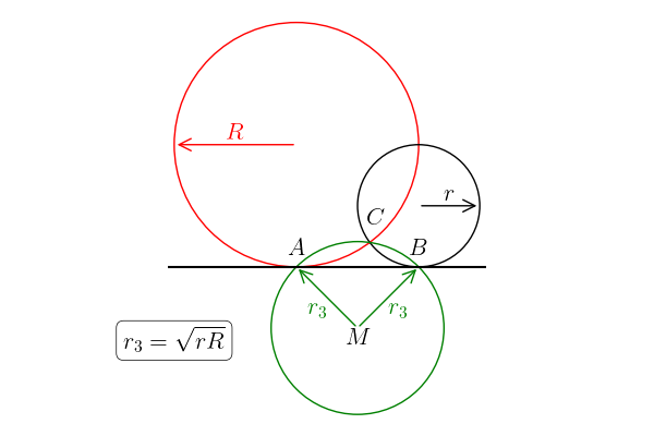
We have three circles, positioned as in Fig.1. The red circle has a radius \(R\) and its center at \((-x, R)\), the black a radius of \(r\) and its center at \((x, r)\). The green circle passes through the three non-collinear points \(A\), \(B\) and \(C\), where \(A\) is the point where the red circle touches the line, \(B\) where the black circle touches the line, and \(C\) the left point of intersection of the red and the black circle. The problem is to prove that the radius \(r_3\) of the green circle is equal to \(\sqrt{rR}\).
I can try to prove this by using some smart reasoning, but why should I?1I had a short chat with my former colleague Jan Willem Polderman in which he challenged me to solve this problem. I recall that Snellius studied the problem to find a circle that goes through three points that are not all three on one line. So, with Snellius’ result, I can conclude that the present problem has a solution, and that I only have to solve the algebra that goes with this. Handling the algebra is a good task for Sagemath, so that is what I am going to use.
As an aside, to print the results nicely, I need the next function.
def Latex(s):
    s = latex(s)
    print(f"\[\n{latex(s)}\n\]")
2. The solution
I first need some variables; \(x, r\) and \(R\) are clear from the problem description. Next, \(-y\) is the \(y\)-coordinate of the center of the green circle; by the symmetry of the figure I have right away that the \(x\)-coordinate of the green circle is \(0\).2To show this is actually the intent of including the two radial vectors in the green circle. Finally, \((u,v)\) are the coordinates of the point \(C\) where all circles intersect.
var('u v r R x', domain='positive')
var('y', domain='real')
With these variables, it is straightforward to solve for \(u\) and \(v\). The point \(C\) lies on the large (red) cicle and on the small (black) circle.
large_circle = (u + x) ^ 2 + (v - R) ^ 2 - R ^ 2
small_circle = (u - x) ^ 2 + (v - r) ^ 2 - r ^ 2
uv_solutions = solve([large_circle, small_circle], u, v, solution_dict=True)
u_sol = uv_solutions[0][u]
v_sol = uv_solutions[0][v]
Latex(u_sol)
Latex(v_sol)
\[ -\frac{2 \, \sqrt{R r - x^{2}} {\left(R - r\right)} x - {\left(R^{2} - r^{2}\right)} x}{R^{2} - 2 \, R r + r^{2} + 4 \, x^{2}} \] \[ \frac{2 \, {\left({\left(R + r\right)} x^{2} - 2 \, \sqrt{R r - x^{2}} x^{2}\right)}}{R^{2} - 2 \, R r + r^{2} + 4 \, x^{2}} \]
The next step is to realize that \(C\) also lies on the green circle. Since, the midpoint of the green circle is \((0, -y)\), and \(C\) has coordinates \((u,v)\), it must be that \((u-0)^{2} + (v-y)^{2} = r^{2}_{3}\). Finally, the point \(B\), with coordinates \((x, 0)\), also lies on the green circle, hence at \((x-0)^{2} + (0-y)^{2} = r_{3}^{2}\). By combining this we can solve for \(y\).
eq = (-y + v_sol) ^ 2 + u_sol ^ 2 == y ^ 2 + x ^ 2
y_solutions = solve(eq, y, solution_dict=True)
y_sol = y_solutions[0][y]
Latex(y_sol)
\[ \frac{2 \, R r - 2 \, x^{2} - \sqrt{R r - x^{2}} {\left(R + r\right)}}{R + r - 2 \, \sqrt{R r - x^{2}}} \]
The last check is to see what expression we get for \(r_3^2 = x^2 + y^2\).
r3_square = x ^ 2 + y_sol ^ 2
Latex(r3_square.simplify_full())
\[ R r \]
So, the result is \(R r\), i.e,. \(r_3^2 = r R\). QED!
3. A simple corollary
Interestingly, when we repeat the computations for the other point at which the red and black intersect, we get the same result!. Here is the proof.
u_sol = uv_solutions[1][u]
v_sol = uv_solutions[1][v]
eq = (-y + v_sol) ^ 2 + u_sol ^ 2 == y ^ 2 + x ^ 2
y_solutions = solve(eq, y, solution_dict=True)
y_sol = y_solutions[0][y]
r3_square = x ^ 2 + y_sol ^ 2
Latex(r3_square.simplify_full())
\[ R r \]
4. Making the figure
Here is the Python code behind Fig.1. With the math above, this is pretty simple.
import matplotlib.pyplot as plt
from matplotlib.patches import Circle
from matplotlib.patches import FancyArrowPatch

plt.rcParams['text.usetex'] = True

r, R = 1.0, 2.0
x = 1.0
y = -1
rR = (x**2 + y**2) ** (0.5)

fig, ax = plt.subplots(figsize=(6, 4))

circle = Circle((-x, R), R, edgecolor='red', facecolor='none')
ax.add_patch(circle)
arrow = FancyArrowPatch(
    (-x, R),
    (-x - R, R),
    arrowstyle='->',
    mutation_scale=20,
    color='red',
    linewidth=1,
)
ax.add_patch(arrow)
ax.text(
    -x - R / 2,
    R,
    r"$R$",
    fontsize=16,
    ha='center',
    va='bottom',
    color='red',
)

circle = Circle((x, r), r, edgecolor='black', facecolor='none')
ax.add_patch(circle)
arrow = FancyArrowPatch(
    (x, r),
    (x + r, r),
    arrowstyle='->',
    mutation_scale=20,
    color='black',
    linewidth=1,
)
ax.add_patch(arrow)
ax.text(
    x + r / 2,
    r,
    r"$r$",
    fontsize=16,
    ha='center',
    va='bottom',
    color='black',
)


circle = Circle((0, y), rR, edgecolor='green', facecolor='none')
ax.add_patch(circle)
arrow = FancyArrowPatch(
    (0, y),
    (x, 0),
    arrowstyle='->',
    mutation_scale=20,
    color='green',
    linewidth=1,
)
ax.add_patch(arrow)
arrow = FancyArrowPatch(
    (0, y),
    (-x, 0),
    arrowstyle='->',
    mutation_scale=20,
    color='green',
    linewidth=1,
)
ax.add_patch(arrow)
ax.text(
    x / 2,
    y / 2,
    r"$r_3$",
    fontsize=16,
    ha='left',
    va='top',
    c='green',
)
ax.text(
    -x / 2,
    y / 2,
    r"$r_3$",
    fontsize=16,
    ha='right',
    va='top',
    c='green',
)


# draw letters A, B, C, M
ax.text(
    -x,
    +0.3,
    r"$A$",
    fontsize=16,
    ha='center',
    va='center',
)
ax.text(
    x,
    +0.3,
    r"$B$",
    fontsize=16,
    ha='center',
    va='center',
)
ax.text(
    0.3,
    +0.8,
    r"$C$",
    fontsize=16,
    ha='center',
    va='center',
)
ax.text(
    0,
    y,
    r"$M$",
    fontsize=16,
    ha='center',
    va='top',
)

# draw theorem
ax.text(
    -x - R,
    y,
    r"$r_3 = \sqrt{r R}$",
    fontsize=16,
    ha='center',
    va='top',
    bbox=dict(
        boxstyle='round', facecolor='white', edgecolor='black', linewidth=0.5
    ),
)


eps = 0.1
ax.plot([-x - R - eps, x + r + eps], [0, 0], color='black')
ax.set_xlim(-x - R - eps, x + r + eps)
ax.set_ylim(-2.5, 2 * R + eps)
ax.axis("off")
ax.set_aspect('equal')

plt.tight_layout()
plt.savefig("../../img/three_circles.png")